Normalizing Flow Maps

Generative modelling with interpolants

Diffusion [9, 18, 19] and flow matching [2, 10, 11] have become the dominant generative modelling paradigm for continuous modalities. Underlying these methods is the idea of defining a time-dependent transport process from a stochastic interpolant [2, 3]: \[ I_t(x_0,x_1):= \alpha_t x_0 + \beta_t x_1 \tag{1}\]

where \(x_0\) is a data sample and \(x_1\) is a noise sample jointly sampled from a coupling distribution \(\pi(x_0,x_1)\), with \(\alpha\) and \(\beta\) well-behaved time-dependent functions. Put simply, given noise and data samples, an interpolant prescribes how we transition from the one to the other.

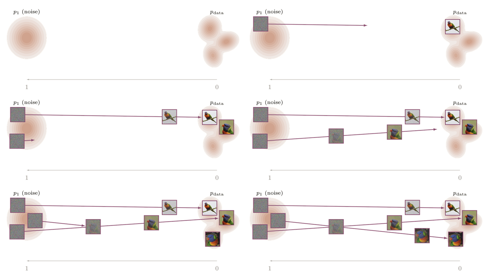
At each time \(t\), sampling pairs \((x_0, x_1)\sim \pi\) and evaluating \(I_t\) gives samples from \(p_t\), the marginal at time \(t\). As \(t\) runs from \(1\) to \(0\), these distributions transform from the noise distribution \(p_1\) to the data distribution \(p_0\):

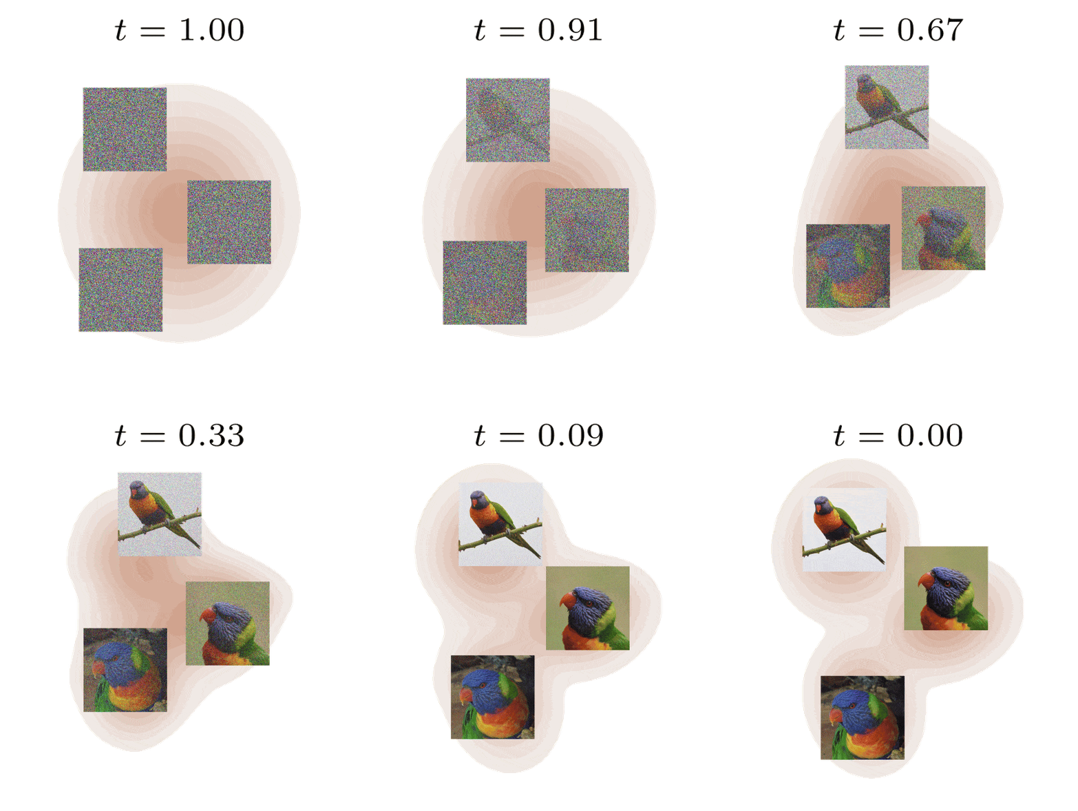
Since sampling from \(p_1\) is easy (by design), a generative model only needs to move samples along this path of distributions from \(p_1\) to \(p_0\). Flow matching and diffusion models do this by learning and then following the velocity field associated with the interpolant: \[ v_t(x) = \mathbb{E}_{x_t\sim p_t(x_t)}\left[\frac{\partial I_t}{\partial t}\vert I_t=x_t\right]. \tag{2}\]

Once a neural network approximation \(v^{\theta}_t\) is learnt, we can sample via \[ \hat{x}_t = x_1 + \int_{\tau=1}^{\tau=t} v^{\theta}_{\tau}(\hat{x}_\tau)d\tau, x_1\sim p_1. \tag{3}\]

This approach produces incredibly high fidelity samples and is scalable as \(v_t\) can be efficiently learnt. In practice, we approximate the integral in Equation 3 with numerical solvers (e.g. Euler). This introduces an inference-time tradeoff where more solver steps can produce better samples at the cost of increasing sampling time. Furthermore, models often require dozens of steps at minimum to obtain reasonable samples. Since each step entails a neural network evaluation this can be quite costly.

Flow maps for efficient sampling

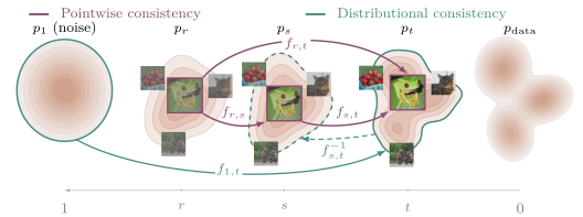
Flow map [4, 5] models instead learn to directly jump along sampling trajectories. Imagine breaking up an integration from \(1\) to \(0\) into an integral up to \(s\), then from \(s\) to \(t\), and finally \(t\) to \(0\):

\[ \hat{x}_0 = \left(\left((x_1 + \int_{\tau=1}^{\tau=s}v_{\tau}(x_\tau)d\tau)+\int_{\tau=s}^{\tau=t}v_{\tau}(x_{\tau})d\tau\right)+\int_{\tau=t}^{\tau=0}v_{\tau}(x_{\tau})d\tau\right) \tag{4}\]

Within each bracket we take the current state and apply some offset by integrating the velocity field over an interval. The flow map \(X_{s,t}\) performs exactly this transformation,

\[ \hat{x}_0 = X_{t,0}(X_{s,t}(X_{1,s}(x_1))). \tag{5}\]

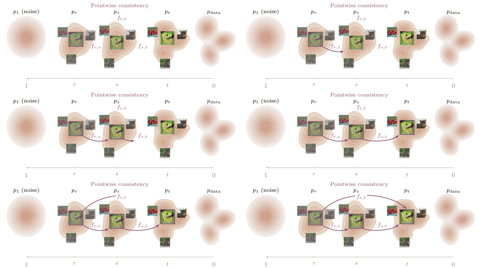
Learning the flow map instead of \(v_t\) enables us to obtain high quality samples in a single step. Flow maps satisfy some intuitively desirable consistency properties which are often directly incorporated into training losses. For example, the semi-group property specifies that composing jumps should be equivalent to a single jump: \[ X_{s,t}(X_{r,s}(x_r)) = X_{r,t}(x_r). \tag{6}\]

What about densities?

Whilst flow maps enable efficient sampling, obtaining exact densities in an efficient way remains challenging. Flow matching models can obtain the log-density of generated samples by integrating the instantaneous change-of-variables formula [6]:

\[ \log p^{\theta}_t(\hat{x}_t) = \log p_1 (x_1) - \int_{\tau=1}^{\tau=t}\nabla\cdot v^{\theta}_{\tau}(\hat{x}_\tau)d\tau. \tag{7}\]

Unfortunately, computing \(\log p^{\theta}_t(\hat{x}_t)\) with sufficient accuracy for scientific applications like Boltzmann Generators requires many solver steps, each needing an expensive velocity field divergence evaluation. Furthermore, directly computing the Fisher score \(\nabla_{\theta}\log p^{\theta}_0(\hat{x}_0)\), a quantity commonly used in reinforcement learning algorithms when rewards are non-differentiable, would require differentiating through the solver steps.

One potential avenue is to simultaneously learn the flow map \(X_{s,t}\) and the integral of the divergence from \(s\) to \(t\). Assuming both quantities are perfectly learnt this would yield cheap and exact densities. However, in practice this is not the case and this approach has so far lagged behind methods that provide exact densities for Boltzmann Generators [1, 14].

A resurgence of normalising flows

Normalising Flows (NFs) [16, 20, 21] parametrize maps between distributions using an invertible neural network \(f^{\theta}\) with Jacobian log-determinants that are cheaply computable. This enables exact and efficient likelihood evaluation via the classical change of variables formula:

\[ \log p^{\theta}_{0}(\hat{x}_0) = \log p_1 (x_1) - \log \left\lvert \mathrm{det} \frac{\partial f^{\theta}(x_1)}{\partial x_1}\right\rvert. \tag{8}\]

NFs are usually trained by maximum-likelihood estimation using \(\log p^{\theta}(x_0) = \log p_1 ((f^{\theta})^{-1}(x_0))+\log \lvert \mathrm{det}\, \partial_{x_0} (f^{\theta})^{-1}(x_0)\rvert\). Whilst NFs provide exact densities, historically they have been difficult to scale and have lagged behind other generative models when it comes to sample fidelity. Recently, Transformer Autoregressive Flows (TARFlows) [8, 12, 23] have emerged as a class of scalable NFs with high quality samples. However, when scaling these NFs to high-dimensional tasks like image generation it is crucial to smooth out the data distribution \(p_0\) via noise injection \[ x_\sigma = x_0 + \epsilon, \,\epsilon \sim \mathcal{N}(0,\sigma^2 I), \tag{9}\]

which prevents training stability issues and poor performance (e.g. Figure 1 below), as well as numerical loss of invertibility.

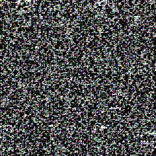
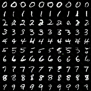
Consequently, the resulting NF provides exact densities for the learnt noisy distribution \(p^{\theta}_{\sigma}\), and clean samples are produced via Tweedie’s formula¹,

\[ \hat{x}_0 = \mathbb{E}[x_0 \vert x_\sigma] = \hat{x}_{\sigma}+\sigma^{2}\nabla_{\hat{x}_{\sigma}}\log p^{\theta}_{\sigma}(\hat{x}_{\sigma}). \tag{10}\]

This additional denoising transformation is not covered by the change-of-variables guarantee and thus the likelihoods of clean samples are not available. Therefore, on high-dimensional data TARFlows lose a key advantage of NFs².

Normalizing Flow Maps

Normalizing Flow Maps (NFMs) perform few-step transport between the marginals \(p_t\) and combine the advantages of NF architectures with an interpolant-centric approach to generative modelling. Given a set of admissible time pairs \(\mathcal{T}\subset \{(s,t): 0\leq t \leq s \leq 1\}\), an NFM is a jointly parametrized family \(\mathcal{F}_{\theta} = {f^{\theta}_{s,t}:\mathbb{R}^{d}\to \mathbb{R}^{d}}_{(s,t)\in \mathcal{T}}\) where for every \((s,t)\in \mathcal{T}\), \(f^{\theta}_{s,t}\) is a \(\mathcal{C}^\infty\) diffeomorphism satisfying

\[ (f_{s,t})^{-1}\circ f_{s,t} = f_{s,t} \circ (f_{s,t})^{-1} = \mathrm{Id}. \tag{11}\]

The exact invertibility of the map enables evaluating sample densities using the classical change-of-variables formula,

\[ \log p^\theta_{s\to t}(x_t) = \log p_s(x_s) - \log\left| \det \frac{\partial f^\theta_{s,t}(x_s)}{\partial x_s} \right|, \qquad x_t=f^{\theta}_{s,t}(x_s),\,x_s\sim p_s. %=(f^\theta_{s,t})^{-1}(x_t). \]

Our first approach, called NFM regression (NFM-R), utilises the sample-level consistency objectives of flow maps to train an NFM. The advantage of NFM-R is that mature training recipes in the flow-map literature (e.g. Mean Flow) can be easily adapted.

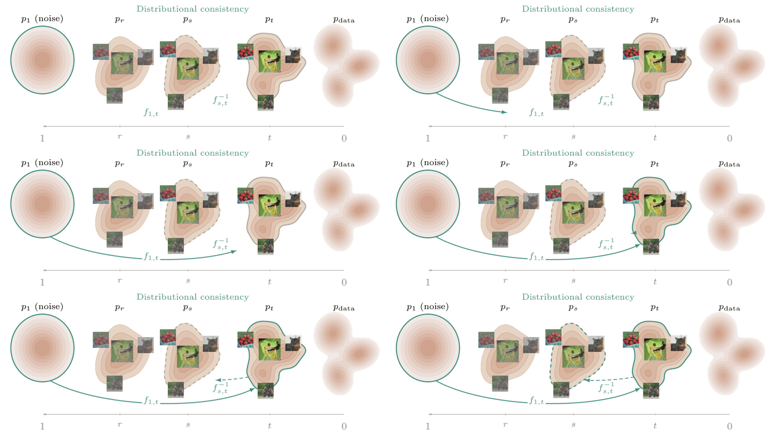
Our second approach, called NFM distribution (NFM-D), performs distributional matching across interpolation times. Our simplest NFM-D objective learns a one-step map from noise to data via: \[ \begin{align} &\operatorname*{argmin}_{\theta} \mathbb{E}_{t,x_0}[\mathbb{D}_{\mathrm{KL}}(p_t(\cdot|x_0)\,\lvert\rvert\,p^{\theta}_{t})]\\ &=\operatorname*{argmin}_{\theta} \mathbb{E}_{t,x_t}\left[\frac{1}{2}\lVert (f^{\theta}_{1,t})^{-1}(x_t) \rVert^2 - \log \left \vert \mathrm{det} \frac{\partial (f^{\theta}_{1,t})^{-1}(x_t)}{\partial x_t}\right \vert\right]. \end{align} \]

Intuitively, this objective teaches the inverse map \((f^{\theta}_{1,t})^{-1}\) to transport samples along an interpolant path back to the noise distribution. Then at inference we can use \(f^{\theta}_{1,t=0}\) to map from noise to data. This is somewhat restrictive as \(f^{\theta}\) can only map from noise, so we don’t benefit from multi-step inference. In the paper, we also detail a more general form of NFM-D that enables multi-step sampling (with densities) at inference.

What can you do with an NFM?

Two applications where NFMs are particularly useful are Reinforcement Learning (RL) post-training and Boltzmann generators.

RL Post-training

For post-training, access to the endpoint density \(p^{\theta}_{1\to 0}(x_0)\) enables direct optimisation of classical regularised reward maximisation objectives, \[ \mathcal{J}(\theta) = \mathbb{E}_{x_0\sim p^{\theta}_{1\to 0}}[R(x_0)] + \beta \mathrm{Reg}(p^{\theta}_{1\to 0}),\, \beta >0. \tag{12}\]

The two most common choices for \(\mathrm{Reg}(p^{\theta}_{1\to 0})\) are entropy \(\mathcal{H}(p^{\theta}_{1\to 0})\) (maximum entropy RL), or \(-\mathbb{D}_{\mathrm{KL}}(p_{1\to 0}^\theta\|p_{\rm ref})\) for a fixed reference density (KL-regularised RL). For diffusion and flow matching models, endpoint likelihoods are expensive to evaluate, making Equation 12 difficult to optimise directly. This necessitates alternative approaches, which are often substantially more complex. NFMs avoid these difficulties as endpoint log densities give access to Fisher score-function gradients (i.e. \(\nabla_{\theta}\log p^{\theta}_{1\to 0}(x_0)\)), which enable learning from non-differentiable rewards, and they provide the density ratios³ needed for prominent large language model post-training methods like DPO [15] and GRPO [17].

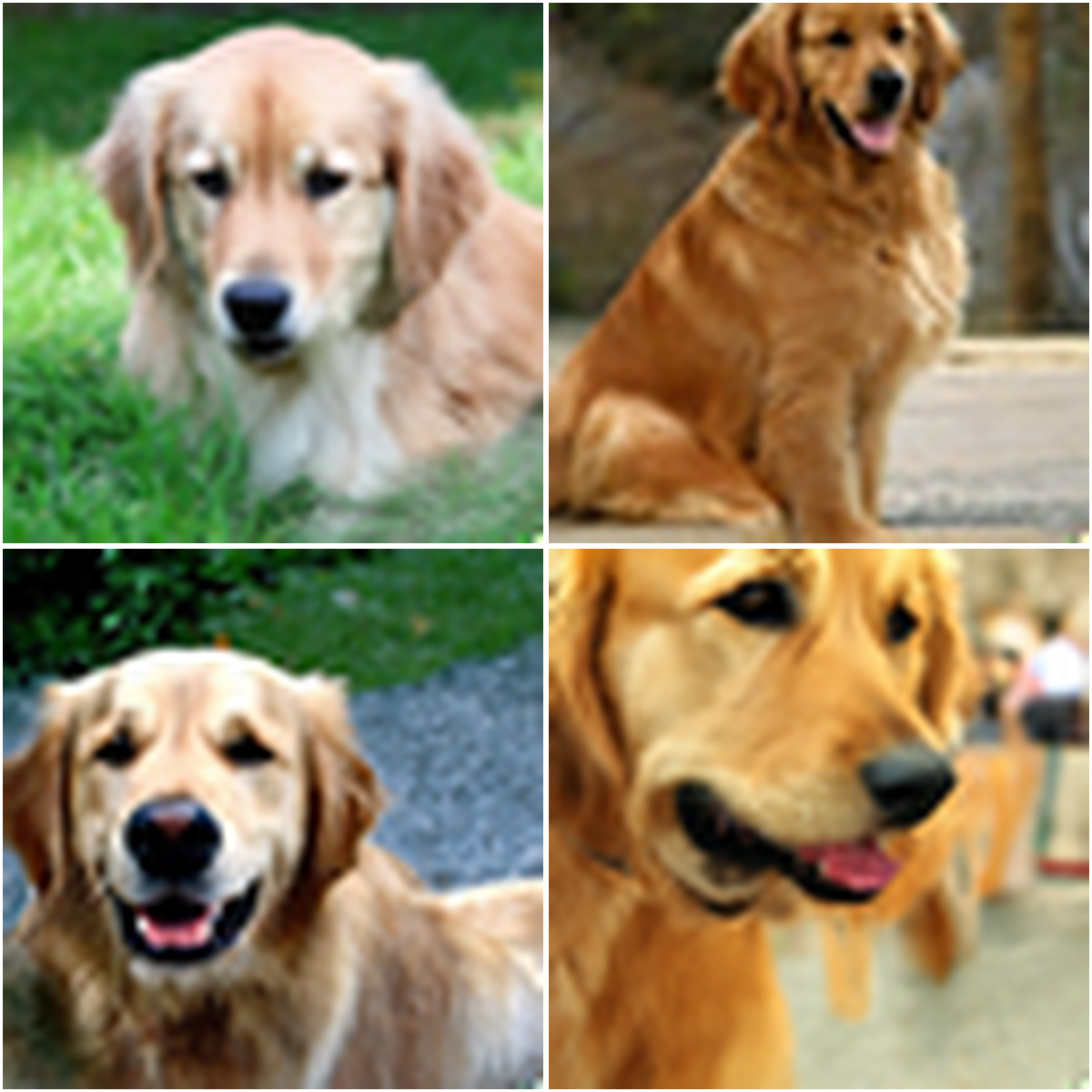
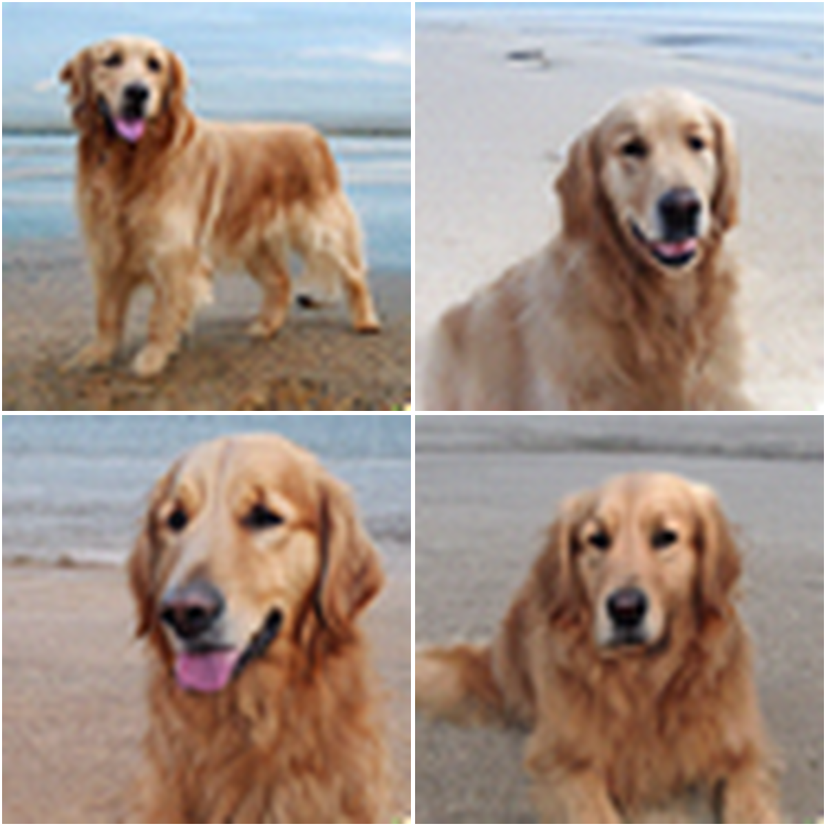
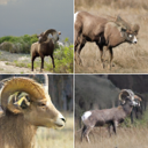
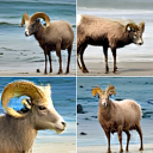
In Figure 2 we demonstrate that purely class-conditional NFM models trained on ImageNet can align their samples with a text-caption supplied to a Visual Language Model (VLM) via on-policy optimisation of Equation 12. NFM-R uses maximum entropy regularisation and pathwise gradients, while we demonstrate the flexibility of NFM-D’s post-training by using KL-regularised REINFORCE.

Boltzmann Generators

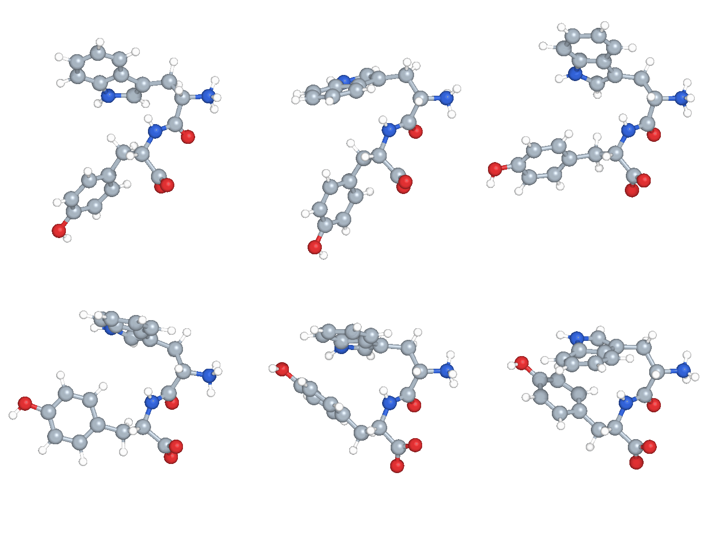
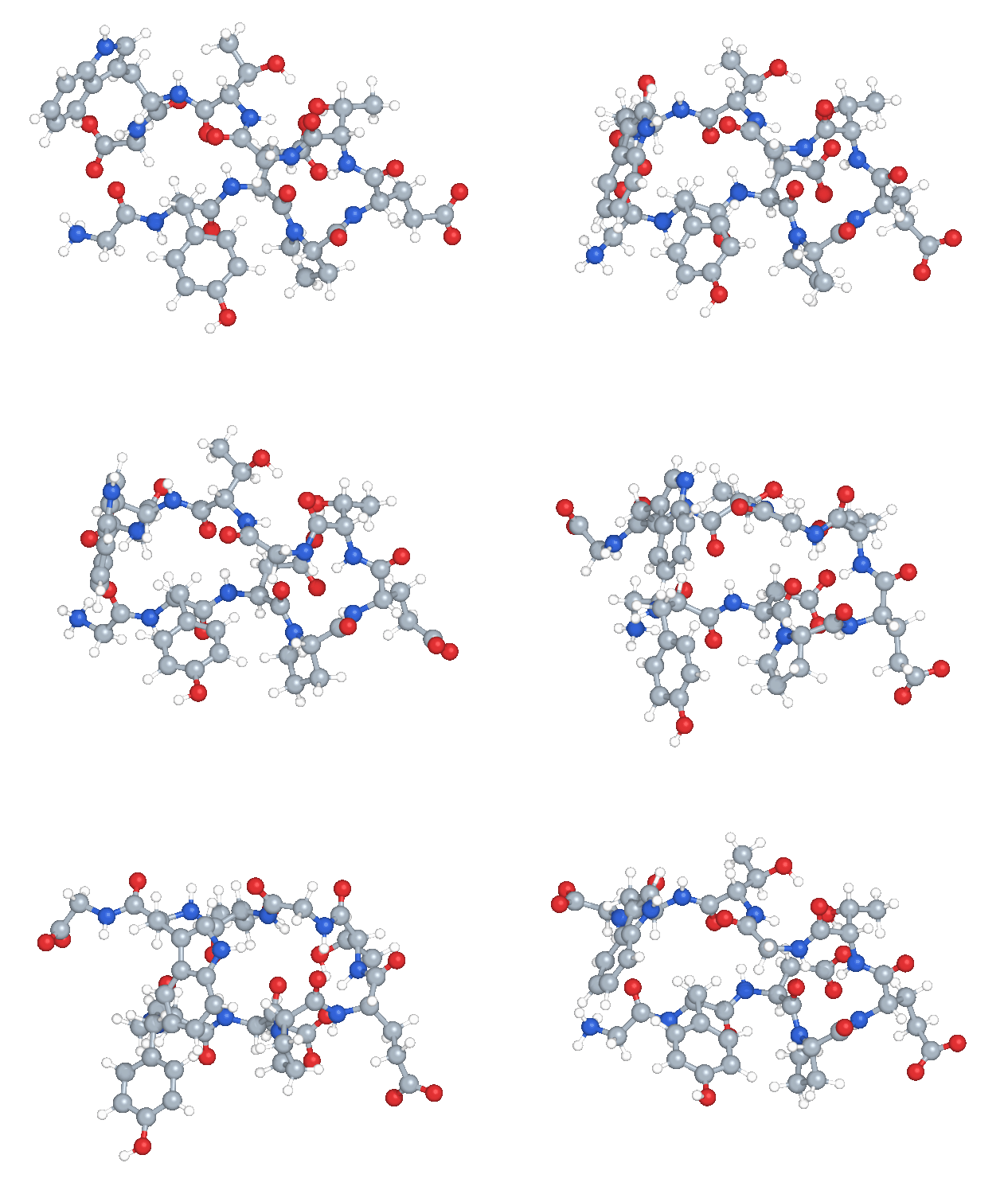
The problem of sampling configurations from equilibrium ensembles is a fundamental problem in statistical physics [7, 22] with applications in biomolecular modeling and drug discovery. For a configuration \(x\) with energy \(\mathcal{E}(x)\) at temperature \(T\), the equilibrium distribution is the Boltzmann distribution \[ \mu_{\mathrm{target}}(x)=\frac{1}{\mathcal{Z}}\exp(-\beta\mathcal{E}(x)),\qquad\mathcal{Z}=\int \exp(-\beta\mathcal{E}(x))dx,\qquad \beta = \frac{1}{k_{B}T}, \]

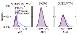
where \(\mathcal{Z}\) is the partition function, which is generally intractable for high-dimensional systems. It is challenging to use traditional methods like Markov Chain Monte Carlo and Molecular Dynamics to sample from the molecular systems that are relevant to areas like drug discovery because their energy landscapes are typically high dimensional and multimodal, with metastable regions separated by large free-energy barriers. Boltzmann Generators (BGs) [13] tackle this problem by learning a generative model that approximates the target Boltzmann distribution and then applying Monte Carlo correction methods (e.g. self-normalised importance sampling) to account for discrepancies between the learned and target distribution. The need for such correction methods entails that BGs must support both efficient sampling and density evaluation.

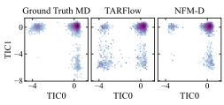
On Chignolin, the most challenging single-peptide benchmark, NFM-D substantially outperforms the best continuous-flow method and matches the current state-of-the-art. Furthermore, on the transferable generation task, which tests zero-shot generalization to unseen peptides, NFM-D consistently beats its MLE-trained TARFlow counterpart and outperforms the current state-of-the-art on five of six metrics.

Closing thoughts

NFMs combine few step sampling with tractable likelihoods and we are particularly excited about their application to post-training and equilibrium sampling. However, they are not without their limitations. NFM-R obtains the highest sample quality on image generation tasks but is prone to becoming numerically non-invertible, which impedes RL methods relying on the Fisher score or KL-regularization. This points to the importance of designing training schemes that enjoy the benefits of both pointwise and distributional consistency.